层标准化

在本教程中，你将编写一个比 PyTorch 实现运行更快的高性能层标准化 (layer normalization) 内核。

在此过程中，你将了解：

在 Triton 中实现反向传播 (backward pass)。
在 Triton 中实现并行归约 (parallel reduction)。

动机

层标准化 (LayerNorm) 算子最先在 BA2016 中提出，旨在提高序列模型（例如 Transformers）或小 batchsize 神经网络的性能。它以向量 $x$ 作为输入，并生成与输入 shape 相同的向量 $y$ 作为输出。标准化是通过减去均值并除以 $x$ 的标准差来实现的。标准化后，会应用带有权重 $w$ 和偏置 $b$ 的可学习线性变换。前向传播可以表示为：

$y = \frac{ x - \text{E}[x] }{ \sqrt{\text{Var}(x) + \epsilon} } * w + b$

其中 $\epsilon$ 是加到分母上的一个小常数，以保证数值稳定性。首先让我们看看前向传播的实现。

import torch
import triton
import triton.language as tl


try:
    # This is https://github.com/NVIDIA/apex, NOT the apex on PyPi, so it
    # should not be added to extras_require in setup.py.
    # 这是 https://github.com/NVIDIA/apex，不是 PyPi 的 apex，
    # 所以不应该加进 setup.py 的额外依赖中
    import apex
    HAS_APEX = True
except ModuleNotFoundError:
    HAS_APEX = False




@triton.jit
def _layer_norm_fwd_fused(
    X,  # pointer to the input 输入指针
    Y,  # pointer to the output 输出指针
    W,  # pointer to the weights 权重指针
    B,  # pointer to the biases 偏差指针
    Mean,  # pointer to the mean 均值指针
    Rstd,  # pointer to the 1/std 1/std 指针
    stride,  # how much to increase the pointer when moving by 1 row 指针移动一行应该增加多少
    N,  # number of columns in X X 的列数
    eps,  # epsilon to avoid division by zero 用于避免除以 0 的 epsilon
    BLOCK_SIZE: tl.constexpr,
):
    # Map the program id to the row of X and Y it should compute.
    # 映射程序 id 到对应计算的 X 和 Y 的行
    row = tl.program_id(0)
    Y += row * stride
    X += row * stride
    # Compute mean
    # 计算均值
    mean = 0
    _mean = tl.zeros([BLOCK_SIZE], dtype=tl.float32)
    for off in range(0, N, BLOCK_SIZE):
        cols = off + tl.arange(0, BLOCK_SIZE)
        a = tl.load(X + cols, mask=cols < N, other=0.).to(tl.float32)
        _mean += a
    mean = tl.sum(_mean, axis=0) / N
    # Compute variance
    # 计算方差
    _var = tl.zeros([BLOCK_SIZE], dtype=tl.float32)
    for off in range(0, N, BLOCK_SIZE):
        cols = off + tl.arange(0, BLOCK_SIZE)
        x = tl.load(X + cols, mask=cols < N, other=0.).to(tl.float32)
        x = tl.where(cols < N, x - mean, 0.)
        _var += x * x
    var = tl.sum(_var, axis=0) / N
    rstd = 1 / tl.sqrt(var + eps)
    # Write mean / rstd
    # 写入 mean / rstd
    tl.store(Mean + row, mean)
    tl.store(Rstd + row, rstd)
    # Normalize and apply linear transformation
    # 归一化并应用线性变换
    for off in range(0, N, BLOCK_SIZE):
        cols = off + tl.arange(0, BLOCK_SIZE)
        mask = cols < N
        w = tl.load(W + cols, mask=mask)
        b = tl.load(B + cols, mask=mask)
        x = tl.load(X + cols, mask=mask, other=0.).to(tl.float32)
        x_hat = (x - mean) * rstd
        y = x_hat * w + b
        # Write output
        tl.store(Y + cols, y, mask=mask)

反向传播

层标准化算子的反向传播比前向传播要复杂一些。

设 $\hat{x}$ 为线性变换前的标准化输入 $\frac{ x - \text{E}[x] }{ \sqrt{\text{Var}(x) + \epsilon} }$ ，那么 $x$ 的向量-雅可比乘积 (VJP) $\nabla_{x}$ 为：

$\nabla_{x} = \frac{1}{\sigma}\Big( \nabla_{y} \odot w - \underbrace{ \big( \frac{1}{N} \hat{x} \cdot (\nabla_{y} \odot w) \big) }_{c_1} \odot \hat{x} - \underbrace{ \frac{1}{N} \nabla_{y} \cdot w }_{c_2} \Big)$

其中 $\odot$ 表示元素逐次相乘， $\cdot$ 表示点积， $\sigma$ 是标准差。 $c_1$ 和 $c_2$ 是中间常数，用于提高以下实现的可读性。

对于权重 $w$ 和偏差 $b$ ，它们的 VJP $\nabla_{w}$ 和 $\nabla_{b}$ 更为简单：

$\nabla_{w} = \nabla_{y} \odot \hat{x} \quad \text{and} \quad \nabla_{b} = \nabla_{y}$

由于在同一批次中的所有行使用相同的权重 $w$ 和偏差 $b$ ，它们的梯度需要累加。为了高效地执行此步骤，我们使用并行归约策略：每个内核实例将某些行的部分 $\nabla_{w}$ 和 $\nabla_{b}$ 累积到 $\text{GROUP\_SIZE\_M}$ 个独立缓冲区之一中。这些缓冲区保存在 L2 缓存中，然后通过另一个函数进一步归约以计算实际的 $\nabla_{w}$ 和 $\nabla_{b}$ 。

设输入行数 $M = 4$ 和 $\text{GROUP\_SIZE\_M} = 2$ ，以下是 $\nabla_{w}$ 的并行归约策略图示（为简洁起见，省略 $\nabla_{b}$ ）：

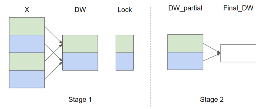
在第一阶段，同色的 X 行共享同一个缓冲区，因此使用 lock 以确保一次只有一个内核实例写入缓冲区。在第二阶段，这些缓冲区会进一步归约以计算最终的 $\nabla_{w}$ 和 $\nabla_{b}$ 。在以下实现中，第一阶段由函数 _layer_norm_bwd_dx_fused 实现，第二阶段由函数 _layer_norm_bwd_dwdb 实现。

@triton.jit
def _layer_norm_bwd_dx_fused(DX,  # pointer to the input gradient 输入梯度指针
                             DY,  # pointer to the output gradient 输出梯度指针
                             DW,  # pointer to the partial sum of weights gradient 权重和梯度指针
                             DB,  # pointer to the partial sum of biases gradient 偏差梯度部分和指针
                             X,  # pointer to the input 输入指针
                             W,  # pointer to the weights 权重指针
                             Mean,  # pointer to the mean 均值指针
                             Rstd,  # pointer to the 1/std 1/std 指针
                             Lock,  # pointer to the lock 锁指针
                             stride,  # how much to increase the pointer when moving by 1 row 指针移动一行应该增加多少
                             N,  # number of columns in X X 的列数
                             GROUP_SIZE_M: tl.constexpr, BLOCK_SIZE_N: tl.constexpr):
    # Map the program id to the elements of X, DX, and DY it should compute.
    # 映射程序 id 到对应计算的 X, DX, DY
    row = tl.program_id(0)
    cols = tl.arange(0, BLOCK_SIZE_N)
    mask = cols < N
    X += row * stride
    DY += row * stride
    DX += row * stride
    # Offset locks and weights/biases gradient pointer for parallel reduction
    # 偏移锁和权重/偏差梯度指针以并行归约
    lock_id = row % GROUP_SIZE_M
    Lock += lock_id
    Count = Lock + GROUP_SIZE_M
    DW = DW + lock_id * N + cols
    DB = DB + lock_id * N + cols
    # Load data to SRAM
    # 读取数据到 SRAM
    x = tl.load(X + cols, mask=mask, other=0).to(tl.float32)
    dy = tl.load(DY + cols, mask=mask, other=0).to(tl.float32)
    w = tl.load(W + cols, mask=mask).to(tl.float32)
    mean = tl.load(Mean + row)
    rstd = tl.load(Rstd + row)
    # Compute dx
    # 计算 ds
    xhat = (x - mean) * rstd
    wdy = w * dy
    xhat = tl.where(mask, xhat, 0.)
    wdy = tl.where(mask, wdy, 0.)
    c1 = tl.sum(xhat * wdy, axis=0) / N
    c2 = tl.sum(wdy, axis=0) / N
    dx = (wdy - (xhat * c1 + c2)) * rstd
    # Write dx
    # 写入 dx
    tl.store(DX + cols, dx, mask=mask)
    # Accumulate partial sums for dw/db
    # 累加 dw 和 db 的部分和
    partial_dw = (dy * xhat).to(w.dtype)
    partial_db = (dy).to(w.dtype)
    while tl.atomic_cas(Lock, 0, 1) == 1:
        pass
    count = tl.load(Count)
    # First store doesn't accumulate
    # 第一个储存不累加
    if count == 0:
        tl.atomic_xchg(Count, 1)
    else:
        partial_dw += tl.load(DW, mask=mask)
        partial_db += tl.load(DB, mask=mask)
    tl.store(DW, partial_dw, mask=mask)
    tl.store(DB, partial_db, mask=mask)
    # Release the lock
    # 释放锁
    tl.atomic_xchg(Lock, 0)




@triton.jit
def _layer_norm_bwd_dwdb(DW,  # pointer to the partial sum of weights gradient 权重部分和指针
                         DB,  # pointer to the partial sum of biases gradient 偏差梯度部分和指针
                         FINAL_DW,  # pointer to the weights gradient 权重梯度指针
                         FINAL_DB,  # pointer to the biases gradient 偏差梯度指针
                         M,  # GROUP_SIZE_M
                         N,  # number of columns 列数
                         BLOCK_SIZE_M: tl.constexpr, BLOCK_SIZE_N: tl.constexpr):
    # Map the program id to the elements of DW and DB it should compute.
    # 映射程序 id 到对应计算的 DW 和 DB
    pid = tl.program_id(0)
    cols = pid * BLOCK_SIZE_N + tl.arange(0, BLOCK_SIZE_N)
    dw = tl.zeros((BLOCK_SIZE_M, BLOCK_SIZE_N), dtype=tl.float32)
    db = tl.zeros((BLOCK_SIZE_M, BLOCK_SIZE_N), dtype=tl.float32)
    # Iterate through the rows of DW and DB to sum the partial sums.
    #迭代通过 DW 和 DB 的行，对部分和进行求和。
    for i in range(0, M, BLOCK_SIZE_M):
        rows = i + tl.arange(0, BLOCK_SIZE_M)
        mask = (rows[:, None] < M) & (cols[None, :] < N)
        offs = rows[:, None] * N + cols[None, :]
        dw += tl.load(DW + offs, mask=mask, other=0.)
        db += tl.load(DB + offs, mask=mask, other=0.)
    # Write the final sum to the output.
    # 将最终结果写入输出
    sum_dw = tl.sum(dw, axis=0)
    sum_db = tl.sum(db, axis=0)
    tl.store(FINAL_DW + cols, sum_dw, mask=cols < N)
    tl.store(FINAL_DB + cols, sum_db, mask=cols < N)

基准测试

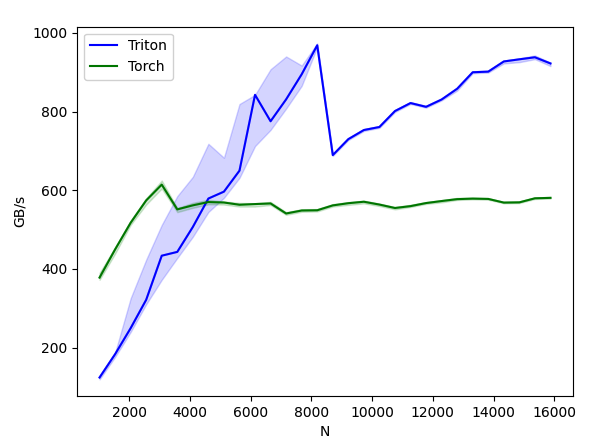
现在我们可以比较 Triton 内核与 PyTorch 的性能了。这里以每个特征少于 64KB 的输入为例进行讲解。具体来说，可以设置 mode: 'backward' 来进行后向传播的基准测试。

class LayerNorm(torch.autograd.Function):


    @staticmethod
    def forward(ctx, x, normalized_shape, weight, bias, eps):
        # allocate output
        # 分配输出
        y = torch.empty_like(x)
        # reshape input data into 2D tensor
        # 将输入数据的形状改为 2D 张量
        x_arg = x.reshape(-1, x.shape[-1])
        M, N = x_arg.shape
        mean = torch.empty((M, ), dtype=torch.float32, device=x.device)
        rstd = torch.empty((M, ), dtype=torch.float32, device=x.device)
        # Less than 64KB per feature: enqueue fused kernel
        # 少于 64KB 每个特征：入队融合内核
        MAX_FUSED_SIZE = 65536 // x.element_size()
        BLOCK_SIZE = min(MAX_FUSED_SIZE, triton.next_power_of_2(N))
        if N > BLOCK_SIZE:
            raise RuntimeError("This layer norm doesn't support feature dim >= 64KB.")
        # heuristics for number of warps
        # 对 warp 数量的启发算法
        num_warps = min(max(BLOCK_SIZE // 256, 1), 8)
        # enqueue kernel
        # 入队内核
        _layer_norm_fwd_fused[(M, )](  #
            x_arg, y, weight, bias, mean, rstd,  #
            x_arg.stride(0), N, eps,  #
            BLOCK_SIZE=BLOCK_SIZE, num_warps=num_warps, num_ctas=1)
        ctx.save_for_backward(x, weight, bias, mean, rstd)
        ctx.BLOCK_SIZE = BLOCK_SIZE
        ctx.num_warps = num_warps
        ctx.eps = eps
        return y


    @staticmethod
    def backward(ctx, dy):
        x, w, b, m, v = ctx.saved_tensors
        # heuristics for amount of parallel reduction stream for DW/DB
        # 计算对 DW/DB 并行规约流数量的启发算法
        N = w.shape[0]
        GROUP_SIZE_M = 64
        if N <= 8192: GROUP_SIZE_M = 96
        if N <= 4096: GROUP_SIZE_M = 128
        if N <= 1024: GROUP_SIZE_M = 256
        # allocate output
        # 分配输出
        locks = torch.zeros(2 * GROUP_SIZE_M, dtype=torch.int32, device=w.device)
        _dw = torch.zeros((GROUP_SIZE_M, N), dtype=x.dtype, device=w.device)
        _db = torch.zeros((GROUP_SIZE_M, N), dtype=x.dtype, device=w.device)
        dw = torch.empty((N, ), dtype=w.dtype, device=w.device)
        db = torch.empty((N, ), dtype=w.dtype, device=w.device)
        dx = torch.empty_like(dy)
        # enqueue kernel using forward pass heuristics
        # 使用前向传播启发算法入队内核
        # also compute partial sums for DW and DB
        # 同样用于计算 DW 和 DB 的部分和
        x_arg = x.reshape(-1, x.shape[-1])
        M, N = x_arg.shape
        _layer_norm_bwd_dx_fused[(M, )](  #
            dx, dy, _dw, _db, x, w, m, v, locks,  #
            x_arg.stride(0), N,  #
            BLOCK_SIZE_N=ctx.BLOCK_SIZE,  #
            GROUP_SIZE_M=GROUP_SIZE_M,  #
            num_warps=ctx.num_warps)
        grid = lambda meta: [triton.cdiv(N, meta['BLOCK_SIZE_N'])]
        # accumulate partial sums in separate kernel
        # 在单独的内核中累加部分和
        _layer_norm_bwd_dwdb[grid](
            _dw, _db, dw, db, min(GROUP_SIZE_M, M), N,  #
            BLOCK_SIZE_M=32,  #
            BLOCK_SIZE_N=128, num_ctas=1)
        return dx, None, dw, db, None




layer_norm = LayerNorm.apply




def test_layer_norm(M, N, dtype, eps=1e-5, device='cuda'):
    # create data
    # 创建数据
    x_shape = (M, N)
    w_shape = (x_shape[-1], )
    weight = torch.rand(w_shape, dtype=dtype, device=device, requires_grad=True)
    bias = torch.rand(w_shape, dtype=dtype, device=device, requires_grad=True)
    x = -2.3 + 0.5 * torch.randn(x_shape, dtype=dtype, device=device)
    dy = .1 * torch.randn_like(x)
    x.requires_grad_(True)
    # forward pass
    # 前向传播
    y_tri = layer_norm(x, w_shape, weight, bias, eps)
    y_ref = torch.nn.functional.layer_norm(x, w_shape, weight, bias, eps).to(dtype)
    # backward pass (triton)
    # 反向传播 (triton)
    y_tri.backward(dy, retain_graph=True)
    dx_tri, dw_tri, db_tri = [_.grad.clone() for _ in [x, weight, bias]]
    x.grad, weight.grad, bias.grad = None, None, None
    # backward pass (torch)
    # 反向传播 (torch)
    y_ref.backward(dy, retain_graph=True)
    dx_ref, dw_ref, db_ref = [_.grad.clone() for _ in [x, weight, bias]]
    # 比较
    assert torch.allclose(y_tri, y_ref, atol=1e-2, rtol=0)
    assert torch.allclose(dx_tri, dx_ref, atol=1e-2, rtol=0)
    assert torch.allclose(db_tri, db_ref, atol=1e-2, rtol=0)
    assert torch.allclose(dw_tri, dw_ref, atol=1e-2, rtol=0)




@triton.testing.perf_report(
    triton.testing.Benchmark(
        x_names=['N'],
        x_vals=[512 * i for i in range(2, 32)],
        line_arg='provider',
        line_vals=['triton', 'torch'] + (['apex'] if HAS_APEX else []),
        line_names=['Triton', 'Torch'] + (['Apex'] if HAS_APEX else []),
        styles=[('blue', '-'), ('green', '-'), ('orange', '-')],
        ylabel='GB/s',
        plot_name='layer-norm-backward',
        args={'M': 4096, 'dtype': torch.float16, 'mode': 'backward'},
    ))
def bench_layer_norm(M, N, dtype, provider, mode='backward', eps=1e-5, device='cuda'):
    # create data
    # 创建数据
    x_shape = (M, N)
    w_shape = (x_shape[-1], )
    weight = torch.rand(w_shape, dtype=dtype, device=device, requires_grad=True)
    bias = torch.rand(w_shape, dtype=dtype, device=device, requires_grad=True)
    x = -2.3 + 0.5 * torch.randn(x_shape, dtype=dtype, device=device)
    dy = .1 * torch.randn_like(x)
    x.requires_grad_(True)
    quantiles = [0.5, 0.2, 0.8]


    def y_fwd():


        if provider == "triton":
            return layer_norm(x, w_shape, weight, bias, eps)  # noqa: F811, E704


        if provider == "torch":
            return torch.nn.functional.layer_norm(x, w_shape, weight, bias, eps)  # noqa: F811, E704


        if provider == "apex":
            apex_layer_norm = (apex.normalization.FusedLayerNorm(w_shape).to(x.device).to(x.dtype))
            return apex_layer_norm(x)  # noqa: F811, E704


    # forward pass
    # 前向传播
    if mode == 'forward':
        gbps = lambda ms: 2 * x.numel() * x.element_size() / ms * 1e-6
        ms, min_ms, max_ms = triton.testing.do_bench(y_fwd, quantiles=quantiles, rep=500)
    # backward pass
    # 反向传播
    if mode == 'backward':
        y = y_fwd()
        gbps = lambda ms: 3 * x.numel() * x.element_size() / ms * 1e-6  # noqa: F811, E704
        ms, min_ms, max_ms = triton.testing.do_bench(lambda: y.backward(dy, retain_graph=True), quantiles=quantiles,
                                                     grad_to_none=[x], rep=500)
    return gbps(ms), gbps(max_ms), gbps(min_ms)




test_layer_norm(1151, 8192, torch.float16)
bench_layer_norm.run(save_path='.', print_data=True)

Out:

layer-norm-backward:

N	Triton	Torch
1024.0	124.121216	378.092307
1536.0	183.402983	449.560983
2048.0	249.502537	517.389457
2560.0	321.675394	574.205608
3072.0	433.694119	614.400016
3584.0	443.381459	551.384634
4096.0	506.721668	561.737163
4608.0	579.015709	570.061876
5120.0	596.504863	568.888888
5632.0	649.846161	563.200014
6144.0	842.605744	564.965499
6656.0	775.456322	566.468098
7168.0	831.072445	540.981122
7680.0	894.757295	548.571433
8192.0	968.512300	549.184373
8704.0	689.425724	561.548373
9216.0	729.980179	567.138460
9728.0	753.135476	570.836186
10240.0	760.866907	563.669722
10752.0	801.391287	554.941947
11264.0	821.689964	559.701851
11776.0	812.137928	567.518063
12288.0	830.738036	572.644636
12800.0	858.100582	577.443635
13312.0	899.966206	578.782596
13824.0	901.565197	578.006963
14336.0	927.396222	568.700819
14848.0	932.858643	569.252402
15360.0	938.015280	579.622631
15872.0	922.343822	580.682936

参考文献

[BA2016] Jimmy Lei Ba and Jamie Ryan Kiros and Geoffrey E. Hinton, “Layer Normalization”, Arxiv 2016

Download Jupyter notebook: 05-layer-norm.ipynb

Download Python source code: 05-layer-norm.py

Download zipped: 05-layer-norm.zip

动机​

反向传播​

基准测试​

参考文献​

动机

反向传播

基准测试

参考文献